By some measures, AI systems are now competitive with traditional computing methods for generating weather forecasts. Because their training penalizes errors, however, the forecasts tend to get “blurry”—as you move further ahead in time, the models make fewer specific predictions since those are more likely to be wrong. As a result, you start to see things like storm tracks broadening and the storms themselves losing clearly defined edges.
But using AI is still extremely tempting because the alternative is a computational atmospheric circulation model, which is extremely compute-intensive. Still, it’s highly successful, with the ensemble model from the European Centre for Medium-Range Weather Forecasts considered the best in class.
In a paper being released today, Google’s DeepMind claims its new AI system manages to outperform the European model on forecasts out to at least a week and often beyond. DeepMind’s system, called GenCast, merges some computational approaches used by atmospheric scientists with a diffusion model, commonly used in generative AI. The result is a system that maintains high resolution while cutting the computational cost significantly.
Ensemble forecasting
Traditional computational methods have two main advantages over AI systems. The first is that they’re directly based on atmospheric physics, incorporating the rules we know govern the behavior of our actual weather, and they calculate some of the details in a way that’s directly informed by empirical data. They’re also run as ensembles, meaning that multiple instances of the model are run. Due to the chaotic nature of the weather, these different runs will gradually diverge, providing a measure of the uncertainty of the forecast.
At least one attempt has been made to merge some of the aspects of traditional weather models with AI systems. An internal Google project used a traditional atmospheric circulation model that divided the Earth’s surface into a grid of cells but used an AI to predict the behavior of each cell. This provided much better computational performance, but at the expense of relatively large grid cells, which resulted in relatively low resolution.
For its take on AI weather predictions, DeepMind decided to skip the physics and instead adopt the ability to run an ensemble.
Gen Cast is based on diffusion models, which have a key feature that’s useful here. In essence, these models are trained by starting them with a mixture of an original—image, text, weather pattern—and then a variation where noise is injected. The system is supposed to create a variation of the noisy version that is closer to the original. Once trained, it can be fed pure noise and evolve the noise to be closer to whatever it’s targeting.
In this case, the target is realistic weather data, and the system takes an input of pure noise and evolves it based on the atmosphere’s current state and its recent history. For longer-range forecasts, the “history” includes both the actual data and the predicted data from earlier forecasts. The system moves forward in 12-hour steps, so the forecast for day three will incorporate the starting conditions, the earlier history, and the two forecasts from days one and two.
This is useful for creating an ensemble forecast because you can feed it different patterns of noise as input, and each will produce a slightly different output of weather data. This serves the same purpose it does in a traditional weather model: providing a measure of the uncertainty for the forecast.
For each grid square, GenCast works with six weather measures at the surface, along with six that track the state of the atmosphere and 13 different altitudes at which it estimates the air pressure. Each of these grid squares is 0.2 degrees on a side, a higher resolution than the European model uses for its forecasts. Despite that resolution, DeepMind estimates that a single instance (meaning not a full ensemble) can be run out to 15 days on one of Google’s tensor processing systems in just eight minutes.
It’s possible to make an ensemble forecast by running multiple versions of this in parallel and then integrating the results. Given the amount of hardware Google has at its disposal, the whole process from start to finish is likely to take less than 20 minutes. The source and training data will be placed on the GitHub page for DeepMind’s GraphCast project. Given the relatively low computational requirements, we can probably expect individual academic research teams to start experimenting with it.
Measures of success
DeepMind reports that GenCast dramatically outperforms the best traditional forecasting model. Using a standard benchmark in the field, DeepMind found that GenCast was more accurate than the European model on 97 percent of the tests it used, which checked different output values at different times in the future. In addition, the confidence values, based on the uncertainty obtained from the ensemble, were generally reasonable.
Past AI weather forecasters, having been trained on real-world data, are generally not great at handling extreme weather since it shows up so rarely in the training set. But GenCast did quite well, often outperforming the European model in things like abnormally high and low temperatures and air pressure (one percent frequency or less, including at the 0.01 percentile).
DeepMind also went beyond standard tests to determine whether GenCast might be useful. This research included projecting the tracks of tropical cyclones, an important job for forecasting models. For the first four days, GenCast was significantly more accurate than the European model, and it maintained its lead out to about a week.
One of DeepMind’s most interesting tests was checking the global forecast of wind power output based on information from the Global Powerplant Database. This involved using it to forecast wind speeds at 10 meters above the surface (which is actually lower than where most turbines reside but is the best approximation possible) and then using that number to figure out how much power would be generated. The system beat the traditional weather model by 20 percent for the first two days and stayed in front with a declining lead out to a week.
The researchers don’t spend much time examining why performance seems to decline gradually for about a week. Ideally, more details about GenCast’s limitations would help inform further improvements, so the researchers are likely thinking about it. In any case, today’s paper marks the second case where taking something akin to a hybrid approach—mixing aspects of traditional forecast systems with AI—has been reported to improve forecasts. And both those cases took very different approaches, raising the prospect that it will be possible to combine some of their features.
Nature, 2024. DOI: 10.1038/s41586-024-08252-9 (About DOIs).